Colors are our embeddings of light
Despite producing and consuming natural language, any large language model needs a way to digest text and to encode/decode it. In the simplest approaches, the first step of this digestion is chunking the input text submitted by the user into a collection of subwords (text chunks), which get mapped to specific scalar values according to certain techniques. These scalars are called tokens, and this process is known as tokenization: it typically employs revisited versions of known encoding techniques which are way older than LLMs, such as byte-pair encoding (introduced in 1994 and repurposed for language models only much later).
What the tokenization algorithm produces is a dictionary subword → scalar, which is called the vocabulary. When reading natural language, the model “speaks” the vocabulary it uses, so it is capable of encoding the sentence it reads into a sequence of integers, by chunking the sentence into the subwords it knows and mapping each subword to the associated scalar.
However, the model still cannot work with these scalars directly: being a single integer value, each of them is too poor an encoding of the processed subword, and the assignment of a scalar to each subword is purely arbitrary, depending only on the training text and on the deterministic tokenization algorithm. The ideal representation of each subword in the vocabulary should be multidimensional and float-based, so that during the training loop the model can adjust the entries of this vectorial representation, learning the best encoding of each subword while chasing the best score in its target function. For this reason, each token in the vocabulary is associated with a vector, called its embedding, and this allows us to represent the whole vocabulary as a stack of these vectors (hence, a matrix \(E \in \mathbb{R}^{M \times d}\), with \(M\) the vocabulary size and \(d\) the number of entries of each vector), where the token associated with a certain subword acts as a row index, selecting the associated vectorial representation.
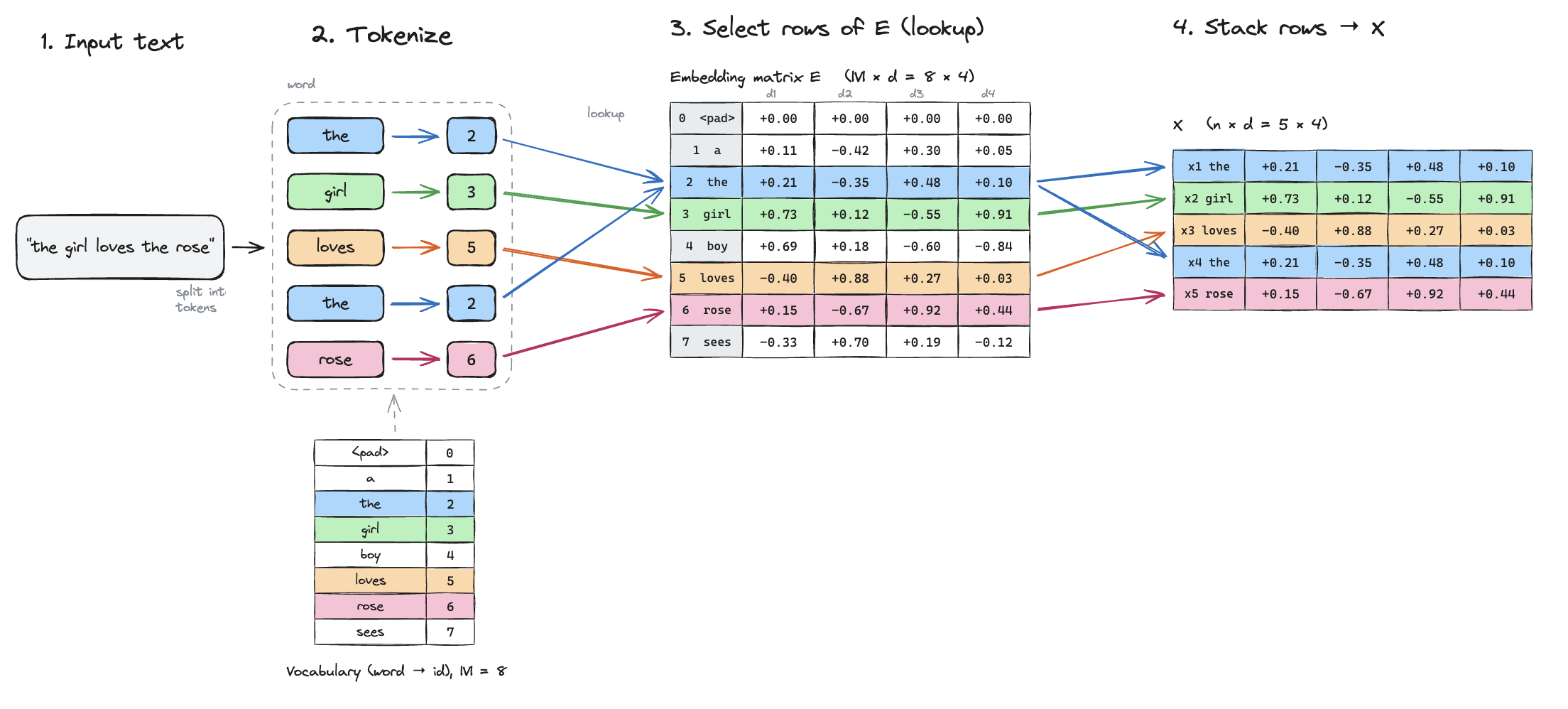
Thus, via tokens and embeddings the model is capable of mapping each input sentence written in natural language into a more or less numerous set of vectors, and their number depends on the tokenization process itself. If there are just a few vectors, we could think of them as an “efficient encoding” of the input sentence, since we have a mathematical encoding of the sentence with just a few vectors. This, however, means that each token covers a big chunk of the sentence, so the vocabulary is probably made of a huge number of tokens and its memory size is probably enormous (given that each vector has hundreds or thousands of entries). On the contrary, if the vocabulary size is very small, we end up with an encoding of the input sentence made of many vectors, hence with more “busy” memory and more operations during the inference pass. Any good tokenization algorithm tries to balance this trade-off associated with the vocabulary size.
The token is an encoding of the subword, typically fixed upfront, before the actual training of the model, while the embedding is the learned feature associated with the subword, that is, the answer of the model to the very natural question: “how do I encode this thing so that, by processing it through my layers, I can score better at my end goal?”.
This is similar to how in linear models you transform the original data in a way that is propaedeutic to the end goal of guessing the final variable. In this context, the transformation is obtained by using the input token as an index in a dictionary lookup, so even if the token scalar itself doesn’t appear in any algebraic transformation leading to the associated embedding, the embedding can still be considered as the “learned image” associated with the token under a certain mapping (in linear models you have \(x \mapsto x\beta\) and the model learns \(x\beta\) by learning \(\beta\); here instead you have \(x \mapsto E[x]\) and the model learns \(E[x]\) directly).
It is fascinating to think about the embedding vector as the “meaning” attached by the model to that subword, not as a claim about the “true, real, absolute” hidden nature of the subword it is dealing with, but rather as something that makes sense to the model and is purely instrumental in modelling the way humans speak, so that it can make better predictions about the words that will follow the input text. Thus, by embedding each subword of the vocabulary it knows, the model creates an “embedding space” which models human speech, trying to capture what is relevant for the objective of guessing which word will follow the input text.
In order to develop an intuition of embeddings as a mathematical, lossy and instrumental encoding of what is experienced by the model, I find it very cool to put them in relation with human sight, since models (via tokenization and embedding) and humans (via eyes and visual brain cortex) follow similar patterns in experiencing an external source and modelling it so that it becomes instrumental in scoring well at a certain goal. The training loop of the model costs gazillions of dollars and aims at text prediction, while for humans the training loop has been going on for millions of years and, as for any other species on the planet, aims at maximizing reproductive success as its end goal.
Light and cone cells
We could say that colors don’t exist in nature as an autonomous physical property of objects: they are what we experience when our visual system encodes and interprets the light reflected by the things we are looking at.
Light as a spectrum
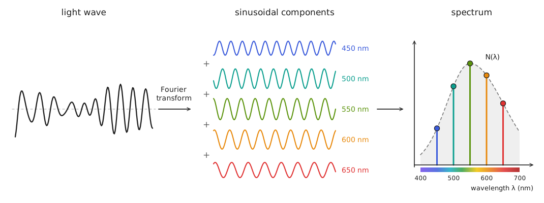
As a very short and terribly inaccurate primer: light is an electromagnetic wave that can be decomposed, through a Fourier transform, into a continuous sum of sinusoidal components, each with its own wavelength. The collection of these components, with their different wavelengths, defines the spectrum of the light source. Photons are distributed across this spectrum, but not all the wavelengths in it can be processed by every organism’s eyes. Different organisms may differ in which wavelengths they can detect.
Cone cells
In organisms with cone-based color vision, the light is captured by cone cells, and humans have around 6 million of these cone-shaped cells across the retina. Despite this huge number, these cells belong to just a few cone types: humans have three of them, so we are considered trichromatic organisms (from the Greek tri = 3 and chroma = color), like honeybees, while dogs and cats have just two and so they are considered dichromatic.
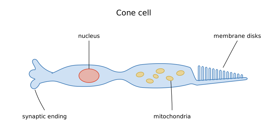
What distinguishes one cone type from another is its sensitivity to photons at different wavelengths, which is typically bell-shaped: a cone type is very good at capturing photons within a certain range of wavelengths, and it gets worse and worse as we move away from that range. The three cone types of humans are conventionally referred to as:
- \(s\), for the cone type that is more sensitive to short wavelengths (i.e., closer to violet), peaking at around 420 nm;
- \(m\), for the cone type that is more sensitive to medium wavelengths, peaking at around 530 nm;
- \(l\), for the cone type that is more sensitive to long wavelengths, peaking at around 560 nm.
These sensitivities are also the reason why we can see only a certain range of wavelengths, approximately from 380 nm to 780 nm: wavelengths below this range (ultraviolet) and above it (infrared) fall in the far tails of the sensitivity curves, so our cone cells are very bad at capturing those photons, if they capture them at all.
At the lower end of this range we find violet wavelengths; wavelengths below it define the ultraviolet (UV) range, typically associated with skin aging, sunburns, and vitamin D synthesis. UV wavelengths are mostly invisible to the human eye, but they are visible to pigeons, goldfish, bees, and many other animals, simply because their cones have different sensitivities.
Quantum catches and the problem of univariance
Now, let \(N(\lambda)\) be the number of photons in a tiny wavelength band centered at \(\lambda\), and let \(p_s(\lambda)\), \(p_m(\lambda)\), and \(p_l(\lambda)\) denote the sensitivities of the \(s\), \(m\), and \(l\) cones at wavelength \(\lambda\). We can then compute the expected number of photons captured by each cone type:
\[S = \int N(\lambda)\,p_s(\lambda)\,d\lambda,\qquad M = \int N(\lambda)\,p_m(\lambda)\,d\lambda,\qquad L = \int N(\lambda)\,p_l(\lambda)\,d\lambda.\]These responses are typically called quantum catches: each of them is the expected number of photons captured by a certain cone type from the same light source.
As mentioned, the wavelength only affects the probability that a photon gets absorbed by a certain cone, depending on its sensitivity, but once the photon is absorbed, the information about its wavelength is lost. This problem is known as univariance (Rushton, 1972).
The issue is that the quantum catch is a single number, which is way too little to characterize the light spectrum being processed, so infinitely many different spectra end up producing the same response. For example, if the response \(L\) is very high, we cannot tell whether this is caused by a few photons at wavelengths where the sensitivity of the \(l\) cone peaks, or by a flood of photons at wavelengths that the cone barely absorbs.
This is exactly the reason why a single cone type is not enough and we need the quantum catches produced by each cone type: the same light gets captured differently by cones with different sensitivities, so by comparing their responses we can tell apart spectra that a single cone would confuse.
The embedding vector of light
For this reason, a more informative representation of the absorbed light is a vector collecting the three quantum catches, obtained from a population of cone cells of the three different types:
\[[L,M,S]\in \mathbb{R}^3\]This vector of quantum catches can be considered as the embedding vector through which the light is encoded by a triplet of cone cells of different types (so, an embedding with just \(d = 3\) entries). In this sense, the human retina maps a light spectrum to a point in \(\mathbb{R}^3\): it is a lossy encoding that collects, in a single vector, the expected number of photons absorbed by each cone type in a given neighborhood. This is extremely nice because it gives us a geometrical representation of the color space defined by our cone cells (see this visualization). In the animation below you can play with it: by moving the peak and the spread of the light source, you can see how the three quantum catches change, and so how the point moves in \(\mathbb{R}^3\).
Thus, \([L,M,S]\) is a primitive vectorial representation of the information captured by the human eye from external light: because of the univariance problem, each entry tells us very little when taken alone, but the three entries together provide a good enough representation of the light that has been captured.
This is incredibly similar to what an embedding vector does for a large language model: each coordinate, taken alone, is insufficient to capture the learned information of a certain token, but when grouped with the others, the coordinates provide a good enough representation of it.
Of course, the vector \([L,M,S]\) mitigates the problem of univariance quite a lot, but it is still a lossy encoding: several different light spectra can map to the same point, even if they are a much smaller family than the ones colliding on a single quantum catch. This is why we experience metamerism, that is, we can perceive two very different light spectra as identical. For example, under a certain light source two objects can appear to have the same color because the light they reflect, despite having different spectra, produces the same \([L,M,S]\in\mathbb{R}^3\), and it may be enough to change the light source to see them with different colors.
What is extremely interesting about all this is that we can interpret the color space known to each species as the embedding space of the visible spectrum of light for that species.
The space belongs to the observer
Our color space is a vectorial representation of the external world that our visual system builds from the light reaching our eyes. It is a coordinate system that makes sense to our brain because it emerged over an enormous amount of evolutionary time, shaped by a very practical target function: survival and reproductive success. It gives us an ergonomic, lossy but efficient representation of the light, which is what we need to spot food, such as fruits and young leaves (Regan et al., 2001; Dominy and Lucas, 2001), and threats.
Of course, this embedding space is very specific to humans: it depends on our three cone types, each with its own sensitivity, and also on the rest of our visual system (such as the visual cortex), which decides how these signals get processed and interpreted.
This is similar to what happens with different models trained on the same corpus of text, which end up with different embedding spaces: also in nature the same external source doesn’t necessarily produce the same internal representation across different species, and even the interpretation of the same representation would differ. In this case, the training target can be easily abstracted across most organisms: survive long enough to reproduce. However, the actual relevant environment, in terms of food, threats and related components, differs largely across species, hence producing very different and specialized vision embedding spaces: a fruit, for example, has a very different relevance to a human, a bee, or a goldfish. Over millions of years of evolution, each species has effectively been optimizing its own “version” of the same target function, shaped by the environment it inhabits, so vision has evolved in different directions, producing different ways of encoding and interpreting light, and hence different vision systems and associated embedding spaces.
Goldfish and several bird species, for example, are tetrachromatic, meaning that they have four different cone types: their vision embedding space lives in a higher dimension compared with ours, and this richer internal representation allows them to distinguish a greater variety of light spectra, hence experiencing fewer metamers than us. Honeybees are instead trichromatic like humans, but their visible spectrum extends approximately from 300 nm to 650 nm, and their sensitivity functions are shifted much more toward the ultraviolet: they are essentially blind to red, while being way more sensitive than us to UV wavelengths. For the same reason, there may be animals that can experience colors we cannot even imagine, how crazy is that?
credits: Vasas, Hanley et al., 2024
After all, color is not an intrinsic property of light itself: it is what comes out of our visual system when it builds its own internal representation of the light. This is, to me, the really fascinating connection with large language models. An embedding is not an “objective” or “unambiguous” representation of the external source, but an internal and model-specific representation of it (for an LLM the source is a token in a text corpus, for a visual system it is the light reaching the eye). In both cases, the representation is shaped by the architecture that processes it and by the target that the system has evolved or been trained to optimize. Nobody designed the coordinates of an embedding vector or of an LMS vector so that they correspond to concepts a human can interpret, and a single dimension doesn’t even need to mean something on its own: if the resulting representation happens to be interpretable, this is just a side effect. This teaches us that knowledge can be purely instrumental for a certain goal and, in general, a learned representation of reality is not necessarily a faithful description of reality: rather, it is a way of encoding information that makes sense for the system consuming it.
The evolutionary story of how, over so many years of training, each species developed its own visual embedding space for very practical reasons associated with reproductive success and related subgoals is just so fascinating, and it says something about us as well: experiencing things is the way we learn them and assign them a certain meaning, and we are typically used to consider as “meaning” a “true, absolute and general” hidden truth about the things we deal with, while it actually is a simple, genuine projection of how they are relevant to us in our experience.
Sharing is caring!


