<?xml version="1.0" encoding="utf-8"?><feed xmlns="http://www.w3.org/2005/Atom" ><generator uri="https://jekyllrb.com/" version="3.10.0">Jekyll</generator><link href="https://fedemagnani.github.io/feed.xml" rel="self" type="application/atom+xml" /><link href="https://fedemagnani.github.io/" rel="alternate" type="text/html" /><updated>2026-05-24T15:35:58+00:00</updated><id>https://fedemagnani.github.io/feed.xml</id><title type="html">Federico Magnani’s blog</title><subtitle>Rust, Computational Mathematics, Finance and other stuff. God bless pane &amp; olio.</subtitle><entry><title type="html">Fork your conversations and rebase your prompts</title><link href="https://fedemagnani.github.io/cs/2026/05/24/fork-your-conversations-and-rebase-your-prompts.html" rel="alternate" type="text/html" title="Fork your conversations and rebase your prompts" /><published>2026-05-24T00:00:00+00:00</published><updated>2026-05-24T00:00:00+00:00</updated><id>https://fedemagnani.github.io/cs/2026/05/24/fork-your-conversations-and-rebase-your-prompts</id><content type="html" xml:base="https://fedemagnani.github.io/cs/2026/05/24/fork-your-conversations-and-rebase-your-prompts.html"><![CDATA[<p>One of the skillsets that the AI phenomenon has quietly boosted is the capability of <strong>explaining yourself</strong>: putting into words what you actually want, and providing methodologies that can unambiguously verify the implementation against your expectations. Turns out that if you can’t describe your intent in a way that survives a stranger reading it cold, the agent can’t either. The good news is that this skill compounds. The bad news is that most of us discover we suck at it the first time we type a prompt and the agent produces something that sounds aligned with your intent, but is fragile and full of disliked side effects.</p>
<h2 id="your-prompt-is-a-lossy-encoding-of-your-intent">Your prompt is a lossy encoding of your intent</h2>

<p>The agent’s job, stripped to its bones, is to infer your intent from very limited sources. Your intent is the real message: rich, fuzzy, packed with implicit context you take for granted. <strong>Your prompt is just its encoding</strong>, and it is almost always a lossy compression of that intent. You, as the user, are also the encoder of this message, and that means you carry the responsibility of encoding it properly to increase the chances of an accurate decoding on the other side. Nobody else is going to do this job for you, and the agent certainly can’t read your mind no matter how many parameters it has.</p>

<p>By default, most agents try to amplify the signal of your prompt by evaluating contextual information around it: the folder you are currently working on, the previous messages exchanged, system prompts, user-defined skills and rules. When this contextual scaffolding is solid and your prompt has high quality, the amplification works in your favor and the agent reconstructs something close to your original intent. When it isn’t, things fall apart in spectacular ways: if the surrounding context is low quality, and/or your prompt is noisy due to vagueness and contradictions, what gets amplified is <strong>noise</strong>. The output is then the canonical AI slop: confident, plausible-looking, and structurally wrong.</p>

<p>The upshot is that agentic engineering requires actual effort to safeguard the quality of prompts and contextual information, and this is not as easy as it might sound. There are a lot of blind spots and missing pre-requisites for an external listener hearing your idea for the first time, and you, while pitching your intent, might genuinely fail to guess all of the information that is missing on the other side. <strong>You can’t audit something you don’t know is missing</strong>. Typically, this gap is handled naturally during the conversation thread, but only on one condition: that the agent is proactively encouraged to be opinionated about your ideas and to raise questions when it feels unsure. Without that nudge, it will happily fill the void with plausible guesses, and you will only notice once the implementation is already on fire.</p>
<h3 id="ask-for-agent-feedback">Ask for agent feedback</h3>
<p>When you are encoding your message (i.e. writing your prompt) you are inevitably estimating which information the agent will need in order to decode it, but your estimate can fail in exhaustivity. So asking the agent for feedback on how confident it is in understanding your intent is essentially asking for a <strong>residual</strong>: the gap between what you transmitted and what the agent actually needed. That residual is valuable information for you, because it tells you exactly where your encoding leaks, and it is typically used in follow-up messages to clarify your intentions and patch the missing bits.</p>
<h3 id="the-problem-of-clarifying-your-intent-with-multiple-prompts">The problem of clarifying your intent with multiple prompts</h3>

<p>This approach is very workable, but it has a cost. Your message (your intent) ends up diluted across multiple lossy encodings (multiple messages), and while effective, this is quite inefficient because it erodes a fundamental budget constraint in agentic engineering: the <strong>context window</strong>. After a long conversation thread the agent will start context-rotting, and this will probably kill the quality of the agentic contribution. Worse, encoding your intent across multiple prompts also lowers the quality of the contextual information that the agent will lean on in the future, when it tries to amplify the signal from the next messages: the past noise is now part of the surrounding context. The takeaway is that <strong>high-quality prompts generate positive externalities both for the current implementation and for the related follow-ups down the line</strong>.</p>
<h2 id="dont-reply-rewind-fork-your-conversation">Don’t reply, rewind: fork your conversation</h2>

<p>In order to mitigate this, I started doing a stupid-simple thing that improved the quality of agentic contributions a lot. I just append the following at the end of my prompt:</p>

<blockquote>
  <p>Before starting the conversation, return your confidence level in the assignment understanding. If it is below 100%, tell me which clarifications you need (if any) and if you have divergent ideas (if any) be opinionated about it, otherwise start the implementation.</p>
</blockquote>

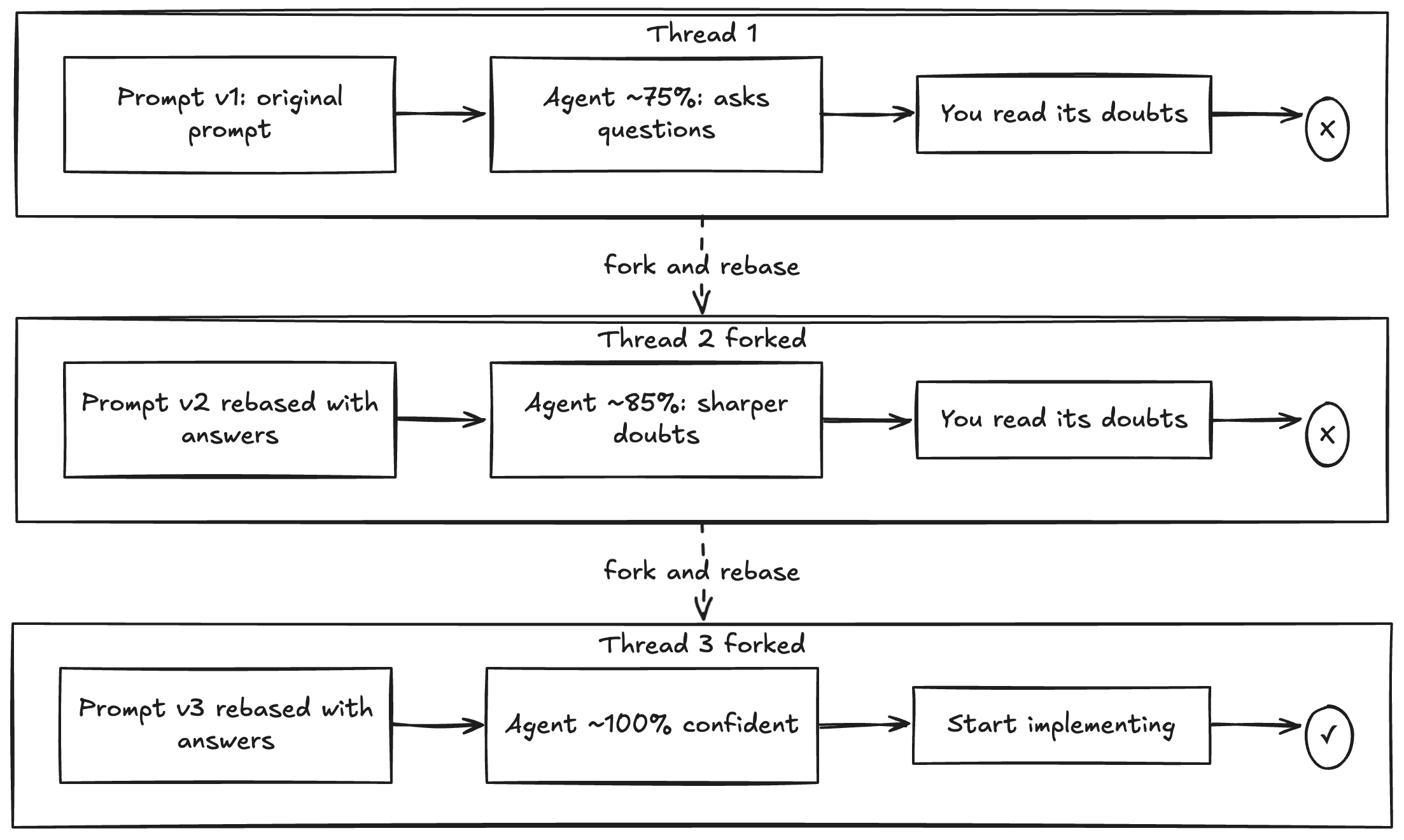
<p>I noticed that the agent will typically answer that it is ~75/80% sure most of the time. While this is obviously a hand-wavy heuristic (what makes a confidence level 70% vs 80%, really?), it forces the agent to stop and focus on the questions that, if left unanswered, would simply get interpreted on the fly. It is like the agent self-prompting the important assignment requirements during its chain of thought, since amplifying the signal of your prompt is the only tool it has when you haven’t given it enough.</p>

<p>Then, depending on the answer, I would <strong>fork the existing conversation</strong> (so that I don’t lose the previous information-rich context) and <strong>rebase my initial prompt</strong> by answering the questions raised in the previous thread. Then I ask again for feedback on how confident the agent is in understanding the assignment. Hopefully, it now understands more, and the new questions/doubts it raises are more detailed, which in turn forces you to be aware and opinionated about specific design decisions you had been hand-waving about. 
The deprecated conversation gives you a <strong>preview</strong> of how the agent would reason on the task, and the answers it produces are exactly the questions it would otherwise have answered in its own head to sketch an acceptable solution. Given this preview, you can roll back in time by forking your conversation at your poorly-prompted message, fix the prompt with the answers to the questions the agent would have asked itself in the chain of thought, and iterate. After a couple of iterations, you end up with a high-quality prompt that condenses multiple feedback sessions with the agent into a single message, and this tremendously improves the quality of the agentic contribution.</p>

<p><img src="/assets/images/fork-and-rebase.png" alt="fork and rebase" /></p>
<h3 id="cognitive-debt-mitigation">Cognitive debt mitigation</h3>

<p>It is quite satisfying to see how, as your prompt improves, the agent’s questions get refined and more specific around the actual implementation of your idea. By forking your conversation again and again, your <strong>latest fork becomes an extremely high-signal thread of messages</strong>: the context window gets extremely optimized, and your cognitive debt on the project gets mitigated as well, since you are forced to pick real implementation decisions in order to resolve the agent’s doubts about your intent. Moreover, this forces you to proactively think about your implementation and follow along while the code is being generated. This is extremely valuable because it also mitigates the amount of cognitive debt you are borrowing while delegating code generation to the agent. <strong>Cognitive surrender</strong> is, in my opinion, one of the most insidious poisons for your project, and it is extremely important to actively avoid it.</p>
<h3 id="the-acceptable-catch">The acceptable catch</h3>

<p>Of course, this comes with a price tag. <strong>You are trading context-window savings for an actual economic cost</strong>, because you are generating output tokens just to reinforce your own prompt. On top of that, <strong>you are spending a non-trivial amount of time “writing English”</strong>, and some people will feel discouraged or get bored quite soon. In my personal experience, and according to my working methodology, I was always happy to pay this trade-off: I found that otherwise the amount of cognitive debt I would collect after an agentic contribution was too high, and I would surrender to AI slop very quickly. I’d rather spend more for a nice contribution than spend slightly less for a miserable one.</p>
<h2 id="closing-thoughts-agentic-engineering-vs-vibe-coding">Closing thoughts: Agentic engineering vs vibe coding</h2>

<p>I think this is what really distinguishes agentic engineering from vibe coding: the involvement and the awareness of the programmer regarding the architectural and practical decisions about the implementation of their intents.</p>

<p>A lazy programmer or a novice will happily borrow cognitive debt to get a quick implementation of their idea while abstracting away the implementation plan entirely, because they are probably chasing a rapid dopamine spike or some feedback about the idea they had in mind: they are not really looking for active engagement with the agent, and they delegate a lot of agency to it regarding the implementation plan, even when this implies immediate or near-future cognitive surrender.</p>

<p>In the context of agentic engineering, instead, this active involvement is what makes the agent a true tool that boosts the user’s skillset, while the user stays in charge of the architectural and implementational decisions of the project. As the user is forced to clarify her own intents, she will probably need to face new domains, and this makes her <strong>hungry</strong> for new information. The cool thing is that you can deep-dive on the reasons why the agent has certain doubts or is opinionated about a certain approach: that new information will be used in the forked conversation rolled back to the original message, and you can deep-dive as much as you want while requesting feedback, since the conversation will be trashed in favor of the forked version anyway.</p>
<h3 id="save-your-boosted-prompts">Save your boosted prompts</h3>

<p>One last habit I would recommend: save each “boosted” prompt. As your project grows, you will collect multiple rich encodings of your intents, and this collection of high-quality prompts might be extremely valuable down the road. Some people even argue that the source code of the future will be equivalent to boosted prompts with a certain structure, so that they can be “compiled” by the agent decoding them, and any coding agent would then be capable of replicating that project most of the time in a programming-language-agnostic fashion. Whether or not you buy that prophecy (probably I am not buyig it to this extent), a <code class="language-plaintext highlighter-rouge">prompts/</code> folder full of well-crafted intents is, at the very minimum, the cleanest documentation of <em>why</em> your project looks the way it does, and might give you a future reference to recall some architectural decisions you made.</p>]]></content><author><name></name></author><category term="cs" /><summary type="html"><![CDATA[One of the skillsets that the AI phenomenon has quietly boosted is the capability of explaining yourself: putting into words what you actually want, and providing methodologies that can unambiguously verify the implementation against your expectations. Turns out that if you can’t describe your intent in a way that survives a stranger reading it cold, the agent can’t either. The good news is that this skill compounds. The bad news is that most of us discover we suck at it the first time we type a prompt and the agent produces something that sounds aligned with your intent, but is fragile and full of disliked side effects. Your prompt is a lossy encoding of your intent]]></summary></entry><entry><title type="html">Necessary but not sufficient conditions are more important than you think</title><link href="https://fedemagnani.github.io/math/2026/05/21/necessary-but-not-sufficient-conditions-are-more-important-than-you-think.html" rel="alternate" type="text/html" title="Necessary but not sufficient conditions are more important than you think" /><published>2026-05-21T00:00:00+00:00</published><updated>2026-05-21T00:00:00+00:00</updated><id>https://fedemagnani.github.io/math/2026/05/21/necessary-but-not-sufficient-conditions-are-more-important-than-you-think</id><content type="html" xml:base="https://fedemagnani.github.io/math/2026/05/21/necessary-but-not-sufficient-conditions-are-more-important-than-you-think.html"><![CDATA[<p>Most of the time when I was reading propositions/theorems/corollaries stating necessary-but-not-sufficient conditions I used to feel almost defrauded: <em>you’re selling me something that sounds useful but actually tells me nothing about the statement I’m trying to prove, since on its own it isn’t enough to prove it.</em></p>

<p>What I’d been missing, though, were several use-cases where knowing a necessary-but-not-sufficient condition can save you:</p>

<ul>
  <li>As a <strong>circuit breaker</strong> in your proof:
    <ul>
      <li>if “N is necessary for P (but may not be sufficient)”, then the moment you realize in your proof that <code class="language-plaintext highlighter-rouge">N==false</code>, you can safely exit early and conclude <code class="language-plaintext highlighter-rouge">P==false</code>.</li>
      <li>if instead <code class="language-plaintext highlighter-rouge">N==true</code>, you still can’t conclude anything about <code class="language-plaintext highlighter-rouge">P</code> (hence my original frustration).</li>
      <li>Under this use case, the necessary-but-not-sufficient condition is extremely useful, paradoxically, when you can prove that it is not satisfied and terribly useless when it is verified</li>
    </ul>
  </li>
  <li>For <strong>piggy-backing</strong> additional properties or statements:
    <ul>
      <li>Suppose that, whether from your proof’s initial assumptions or from something derived along the way, you observe <code class="language-plaintext highlighter-rouge">P==true</code>: trivially, every condition required for <code class="language-plaintext highlighter-rouge">P</code> to exist must hold, otherwise <code class="language-plaintext highlighter-rouge">P</code> couldn’t exist in the first place.</li>
      <li>Consequently, if any prop/theorem/proof states “N is a necessary condition for P (but may not be sufficient)”, then <code class="language-plaintext highlighter-rouge">P==true</code> hands you <code class="language-plaintext highlighter-rouge">N==true</code> for free.</li>
      <li>This is also what the notation <code class="language-plaintext highlighter-rouge">P =&gt; N</code> really means: if <code class="language-plaintext highlighter-rouge">N</code> is a necessary (but perhaps not sufficient) condition for <code class="language-plaintext highlighter-rouge">P</code>, then <code class="language-plaintext highlighter-rouge">P</code> is a sufficient (but perhaps not necessary) condition for <code class="language-plaintext highlighter-rouge">N</code>.</li>
      <li>However, if your aim is to get <code class="language-plaintext highlighter-rouge">N</code> for free but <code class="language-plaintext highlighter-rouge">P==false</code>, then you still can’t say anything about <code class="language-plaintext highlighter-rouge">N</code>.</li>
      <li>In contrast to the previous case, here the necessary-but-not-sufficient condition is incredibly useful (and generous) whenever it applies because of the existence itself of <code class="language-plaintext highlighter-rouge">P</code>, and completely useless when <code class="language-plaintext highlighter-rouge">P==false</code></li>
    </ul>
  </li>
</ul>]]></content><author><name></name></author><category term="math" /><summary type="html"><![CDATA[Most of the time when I was reading propositions/theorems/corollaries stating necessary-but-not-sufficient conditions I used to feel almost defrauded: you’re selling me something that sounds useful but actually tells me nothing about the statement I’m trying to prove, since on its own it isn’t enough to prove it.]]></summary></entry><entry><title type="html">The quadratic sandwich</title><link href="https://fedemagnani.github.io/math/2026/04/08/the-quadratic-sandwich.html" rel="alternate" type="text/html" title="The quadratic sandwich" /><published>2026-04-08T00:00:00+00:00</published><updated>2026-04-08T00:00:00+00:00</updated><id>https://fedemagnani.github.io/math/2026/04/08/the-quadratic-sandwich</id><content type="html" xml:base="https://fedemagnani.github.io/math/2026/04/08/the-quadratic-sandwich.html"><![CDATA[<p>If you have ever tried to minimize a function with gradient descent, you probably noticed that some functions are a joy to optimize and others are a nightmare. The difference often boils down to two properties: <strong>strong convexity</strong> and <strong>L-smoothness</strong>. These two concepts define a “sandwich” of quadratic bounds around your function that tells you <em>exactly</em> how well-behaved it is. If the sandwich is tight, life is good. If one slice of bread is missing, things get ugly fast.</p>

<p>In this post we’ll build up both concepts from scratch, see how they combine into the quadratic sandwich, understand what happens at the level of the Hessian’s eigenvalues, and pick up a neat trick to verify L-smoothness without ever computing an eigenvalue.</p>

<h2 id="strong-convexity--the-function-cant-be-too-flat"><a href="#strong-convexity">Strong convexity — the function can’t be too flat</a></h2>

<p>A differentiable function \(f:\mathbb{R}^n\to\mathbb{R}\) is \(\mu\)-strongly convex (with \(\mu &gt; 0\)) if for all \(x, y\)</p>

\[f(y) \geq f(x) + \langle \nabla f(x), y - x \rangle + \frac{\mu}{2} \|y - x\|^2\]

<p>If this looks familiar, it’s because the first two terms on the right are the first-order Taylor expansion of \(f\) at \(x\). For a plain convex function, the Taylor expansion is already a global underestimator (that’s the subgradient inequality). But strong convexity asks for more: the function must stay above the tangent <em>plus a quadratic gap</em>. The parameter \(\mu\) controls how aggressive this gap is — the bigger \(\mu\), the more the function curves upward and away from its linear approximation.</p>

<p>The intuition is that a strongly convex function has a guaranteed minimum curvature of \(\mu\) in every direction. It can’t flatten out, it can’t plateau, it can’t have a degenerate valley where one direction is basically flat. There is always a force pulling you toward the minimum, and that force grows linearly with the distance from the minimizer.</p>

<div style="overflow:auto; border: 1px solid #ccc;">
    <iframe src="https://www.desmos.com/calculator/wswrrpl586?embed" height="500" style="width: 100%; border: 0;" frameborder="0">
    </iframe>
</div>

<h2 id="l-smoothness--the-function-cant-be-too-steep"><a href="#l-smoothness">L-smoothness — the function can’t be too steep</a></h2>

<p>A differentiable function \(f\) is \(L\)-smooth if its gradient is Lipschitz continuous:</p>

\[\|\nabla f(x) - \nabla f(y)\| \leq L \|x - y\| \quad \forall \; x, y\]

<p>Read this carefully: the change in the gradient between any two points is always dominated by a rescaled version of the change in the input. No matter how far apart \(x\) and \(y\) are, the gradient difference \(\|\nabla f(x) - \nabla f(y)\|\) can never outpace \(L\) times the input difference \(\|x - y\|\). The constant \(L\) acts as a leash on the gradient: it can move, but it can’t jerk. No abrupt turns, no sudden spikes in curvature.</p>

<p>Now here’s the equivalent characterization that will matter for the sandwich, sometimes called the <strong>descent lemma</strong>: if \(f\) is convex and \(L\)-smooth, then for all \(x, y\)</p>

\[f(y) \leq f(x) + \langle \nabla f(x), y - x \rangle + \frac{L}{2}\|y - x\|^2\]

<p>This is not obvious from the Lipschitz condition alone — it requires a short derivation that we work out in the <a href="#appendix-descent-lemma">Appendix</a>. The key idea is to integrate the gradient along the segment from \(x\) to \(y\) and use Cauchy-Schwarz together with the Lipschitz bound to control the error.</p>

<p>Look at the structure: same shape as the strong convexity condition, but with the inequality flipped and \(\mu\) replaced by \(L\). The function now stays <em>below</em> its tangent plus a quadratic term. In other words, the function can bend, but not more than a quadratic with curvature \(L\).</p>

<p>The parameter \(L\) caps the maximum curvature in any direction. If strong convexity sets a floor on curvature, L-smoothness sets a ceiling.</p>

<div style="overflow:auto; border: 1px solid #ccc;">
    <iframe src="https://www.desmos.com/calculator/92wwgqz2qd?embed" height="500" style="width: 100%; border: 0;" frameborder="0">
    </iframe>
</div>

<h2 id="the-quadratic-sandwich"><a href="#the-quadratic-sandwich">The quadratic sandwich</a></h2>

<p>Now we put both slices of bread together. If \(f\) is \(\mu\)-strongly convex <em>and</em> \(L\)-smooth, then both inequalities hold simultaneously and for all \(x, y\) we get</p>

\[\begin{cases}
f(x) + \langle \nabla f(x), y - x \rangle + \frac{\mu}{2}\|y - x\|^2 \leq f(y) \\[6pt]
f(y) \leq f(x) + \langle \nabla f(x), y - x \rangle + \frac{L}{2}\|y - x\|^2
\end{cases}\]

<p>The function is trapped between two parabolas centered at any point \(x\): a tighter one from below (curvature \(\mu\)) and a wider one from above (curvature \(L\)). This is the quadratic sandwich.</p>

<p>The proof of the sandwich is worked out in the <a href="#appendix-descent-lemma">Appendix</a>.</p>

<div style="overflow:auto; border: 1px solid #ccc;">
    <iframe src="https://www.desmos.com/calculator/awzmdi4ehw?embed" height="500" style="width: 100%; border: 0;" frameborder="0">
    </iframe>
</div>

<h3 id="the-condition-number">The condition number</h3>

<p>The ratio</p>

\[\kappa = \frac{L}{\mu}\]

<p>is called the <strong>condition number</strong> and it measures how thick the sandwich is. By construction, since \(L \geq \mu\) (the maximum curvature can’t be smaller than the minimum curvature), the condition number is always bounded below by 1: \(\kappa \geq 1\). A small \(\kappa\) (close to 1) means the function is “almost quadratic” — both bounds are tight, and the function is easy to optimize. A large \(\kappa\) means the curvature varies wildly across directions, and this is where gradient descent starts to suffer. Think about it in two scenarios:</p>

<ul>
  <li><strong>Some directions lack curvature</strong> (\(\mu\) is tiny): a small \(\mu\) doesn’t necessarily mean the function is flat — you could still have a nonzero slope. But it means you have no “acceleration” to exploit: the gradient barely changes from one iterate to the next, so you can’t gauge whether you’re getting closer to the minimum or how to adjust your step size. Think of walking on a constant slope — you’re moving, but the terrain gives you no feedback about your progress.</li>
  <li><strong>The gradient changes too abruptly</strong> (\(L\) is huge): contrary to the lack of strong convexity — where the problem is that the gradient <em>doesn’t</em> change — here the problem is that it changes <em>too much</em>. All of a sudden, between one iterate and the next, the gradient spikes or flips direction in a way that your step size didn’t anticipate. Note that a large \(L\) alone is not necessarily catastrophic: if \(\mu\) is also large (high curvature everywhere), the function is just a steep but well-behaved bowl, and you can simply use a small step size \(1/L\) that works uniformly.</li>
</ul>

<p>The real trouble comes from the <em>spread</em> between \(L\) and \(\mu\) — a large condition number \(\kappa = L/\mu\). When the gap is significant, some directions have high curvature (where the gradient changes fast) and others have low curvature (where the gradient is nearly constant). A single step size cannot serve both: sized for the high-curvature directions it’s too conservative for the low-curvature ones, and vice versa. This mismatch is what causes the classic zigzagging behavior of gradient descent — it’s not \(L\) alone or \(\mu\) alone, but the ill-conditioning between them.</p>

<p>When \(\kappa = 1\) (that is, \(\mu = L\)), the sandwich is perfectly balanced: the same quadratic function bounds \(f\) from above and from below. Since \(f\) is squeezed between two identical parabolas, it must <em>be</em> that parabola. The sandwich collapses into an equality: for all \(x, y\)</p>

\[f(y) = f(x) + \langle \nabla f(x), y - x \rangle + \frac{\mu}{2}\|y - x\|^2\]

<p>The function is <em>exactly</em> its own second-order approximation everywhere — no error, no slack. Now evaluate this at the minimizer \(x^\star\) where \(\nabla f(x^\star) = 0\):</p>

\[f(y) = f(x^\star) + \frac{\mu}{2}\|y - x^\star\|^2\]

<p>So \(f\) is a perfect quadratic bowl centered at \(x^\star\). But we can squeeze out more. Differentiating the equality with respect to \(y\) gives \(\nabla f(y) = \mu(y - x^\star)\): the gradient at any point is just a rescaled vector pointing radially away from the minimizer. There is no zigzagging, no misalignment — gradient descent with step size \(1/\mu\) reaches the minimum in exactly one step:</p>

\[y - \frac{1}{\mu}\nabla f(y) = y - (y - x^\star) = x^\star\]

<p>In other words, the only functions with a perfect sandwich are quadratics, and quadratics are the only functions where gradient descent doesn’t need to iterate at all.</p>

<h2 id="what-goes-wrong-without-one-slice-of-bread"><a href="#what-goes-wrong">What goes wrong without one slice of bread</a></h2>

<h3 id="without-strong-convexity">Without strong convexity</h3>

<p>Set \(\mu = 0\) and the lower bound degenerates into the tangent hyperplane — you lose the quadratic pull toward the minimum. The condition number \(\kappa = L/\mu\) blows up to \(+\infty\), which is the mathematical way of saying “gradient descent is going to have a bad time”.</p>

<p>The secret sauce of strong convexity is that the gradient is guaranteed to change in an appreciable way at every step. For a \(\mu\)-strongly convex function, \(\|\nabla f(x)\|\) grows at least proportionally to \(\|x - x^\star\|\): a big gradient means you’re far from the optimum, a small gradient means you’re close. At every iterate, the gradient norm lets you prelude how close you are to the minimum — it’s a <em>calibrated signal</em>. This has concrete algorithmic consequences: if you know roughly how far you are, you can take appropriately sized steps — large when far, small when close (assuming the field changes smoothly under your feet, which is what L-smoothness guarantees).</p>

<p>Without strong convexity, the gradient loses this calibration. Consider \(f(x) = \|x\|_1\): the gradient is \(\pm 1\) everywhere except the origin — it gives you the direction but says nothing about the distance. Whether you’re at \(x = 100\) or \(x = 0.001\), the gradient screams with the same intensity. The gradient doesn’t change at all as you move, so you have no way to gauge your progress. The same happens with the Huber loss: once you’re in the linear regime, the gradient is constant and you can’t tell if you’re close or far. Without a gradient that scales with the distance, the solver is flying blind — it has no way to modulate its step size based on proximity to the minimum.</p>

<p>Even worse, without strong convexity you lose the guarantee that the minimizer is unique. The function might have a whole subspace of minimizers, or a flat region where the gradient vanishes but you’re nowhere near the optimum.</p>

<!-- DESMOS PLACEHOLDER
**Chart: gradient descent without strong convexity**

Run gradient descent on $$f(x_1, x_2) = \frac{1}{4}(x_1 + x_2)^4$$, which is not strongly convex. The Hessian is $$3(x_1+x_2)^2 \begin{pmatrix} 1 & 1 \\ 1 & 1 \end{pmatrix}$$, which has eigenvalues $$6(x_1+x_2)^2$$ and $$0$$. The zero eigenvalue corresponds to the direction $$(1, -1)$$ (the anti-diagonal): along this direction the function is completely flat. The curvature only exists along $$(1, 1)$$, and it vanishes on the line $$x_1 + x_2 = 0$$.

The gradient is $$\nabla f = ((x_1+x_2)^3,\; (x_1+x_2)^3)$$, so the update rule is:
- $$x_1^{(k+1)} = x_1^{(k)} - \eta \, (x_1^{(k)}+x_2^{(k)})^3$$
- $$x_2^{(k+1)} = x_2^{(k)} - \eta \, (x_1^{(k)}+x_2^{(k)})^3$$

Display:
- Contour lines of $$f$$ in the $$(x_1, x_2)$$ plane (these are parallel strips around the line $$x_1 + x_2 = 0$$)
- The iterates $$(x_1^{(k)}, x_2^{(k)})$$ as dots connected by line segments (e.g. 20-30 iterates)
- The line $$x_1 + x_2 = 0$$ (the set of minimizers) drawn as a dashed line

Sliders:
- $$\eta \in [0.01, 0.5]$$ (step size)
- Starting point draggable or $$(x_1^{(0)}, x_2^{(0)}) = (2, 1)$$

Key behavior: gradient descent moves only along the $$(1, 1)$$ direction (since both gradient components are always equal), approaching the line $$x_1 + x_2 = 0$$ but never sliding along it. The convergence slows down dramatically near the line of minimizers because the curvature vanishes there — the gradient $$(x_1+x_2)^3$$ shrinks cubically. The algorithm converges to $$(\frac{1}{2}, -\frac{1}{2})$$ (the projection of the starting point onto the minimizer line), but the last few iterates barely move. This is the flat direction pathology: no curvature along the kernel direction, and vanishing curvature near the minimizers.
-->

<!-- DESMOS PLACEHOLDER
**Chart: pathology — missing strong convexity (1D)**

Plot $$f(x) = \frac{1}{100}x^4$$:
- The function $$f(x)$$ in bold (red)
- Its first-order approximation at $$a$$: $$\ell_a(x) = f(a) + f'(a)(x - a)$$ (gray dashed), where $$f'(x) = \frac{4}{100}x^3$$
- Attempted strong convexity lower bound: $$q^-_a(x) = f(a) + f'(a)(x-a) + \frac{\mu}{2}(x-a)^2$$ (blue)

Sliders:
- $$a \in [-3,3]$$ (tangent point)
- $$\mu \in [0.01, 1]$$ (attempted strong convexity parameter)

Key behavior: no matter what $$\mu$$ you pick, the blue parabola will eventually poke above the red curve near the origin (where the function is extremely flat). There is no global $$\mu > 0$$ that works.
-->

<div style="overflow:auto; border: 1px solid #ccc;">
    <iframe src="https://www.desmos.com/calculator/uwwlpwydjf?embed" height="500" style="width: 100%; border: 0;" frameborder="0">
    </iframe>
</div>

<!-- <div style="overflow:auto; border: 1px solid #ccc;">
    <iframe src="https://www.desmos.com/3d/arumbpubx6?lang=it" height="800"
        style="width: 100%; border: 0;" frameborder="0">
    </iframe>
</div> -->

<h3 id="without-l-smoothness">Without L-smoothness</h3>

<p>Imagine you’re kicking a ball blindly toward a target — you can’t see the field, but someone tells you the direction to kick. As long as you’re kicking in the mud, life is predictable: the ball moves a little bit each time, the friction keeps things under control, and you can reasonably expect where it will land after each kick. You make steady progress, kick after kick. But now imagine the mud suddenly disappears and you’re on ice. You kick with the same energy as before, but this time the ball flies away — it overshoots the target and lands even further from it than where you started. The ground changed under your feet, but your kicking force didn’t adapt.</p>

<p>That’s the core problem without L-smoothness: you find a step size that works well in one region (where the gradient is moderate, the “mud”), you proceed confidently, but you end up in a region where the gradient has exploded (the “ice”) — the change in the gradient was way bigger than the change in the input. Using the same step size now produces a catastrophic overshoot, and you might end up further from the minimum than where you began.</p>

<p>Mathematically: remove the upper bound and the function is free to spike arbitrarily. A solver that takes a step based on the current gradient has no guarantee about what the function value will be at the new point — it could be much higher than expected because the curvature exploded between the current point and the next.</p>

<p>Consider \(f(x) = -\ln(x)\) for \(x &gt; 0\): the second derivative is \(\frac{1}{x^2}\), which is unbounded as \(x \to 0\). Far from the origin the function is gentle (at \(x = 10\), the curvature is just \(0.01\)), but near the origin the curvature explodes (at \(x = 0.1\), the curvature is \(100\)). A step size calibrated for the gentle region will massively overshoot if it carries you into the steep region, and a step size conservative enough for the steep region will crawl everywhere else.</p>

<p>In the extreme case of a non-differentiable function like \(f(x) = \|x\|\), the gradient changes instantaneously at the kink — the effective \(L\) is infinite at that point. Standard gradient descent simply cannot handle this without modification.</p>

<!-- DESMOS PLACEHOLDER
**Chart: pathology — missing L-smoothness**

Plot $$f(x) = x^4$$:
- The function $$f(x)$$ in bold (red)
- Its first-order approximation at $$a$$: $$\ell_a(x) = f(a) + f'(a)(x - a)$$ (gray dashed), where $$f'(x) = 4x^3$$
- Attempted L-smoothness upper bound: $$Q^+_a(x) = f(a) + f'(a)(x-a) + \frac{L}{2}(x-a)^2$$ (green)

Sliders:
- $$a \in [-3,3]$$ (tangent point)
- $$L \in [1, 50]$$ (attempted smoothness parameter)

Key behavior: for any fixed $$L$$, move the tangent point $$a$$ far from the origin and the green parabola will fail to stay above the red curve. The function always escapes the upper bound eventually. No finite $$L$$ works globally.
-->

<div style="overflow:auto; border: 1px solid #ccc;">
    <iframe src="https://www.desmos.com/calculator/knzwn4w2tk?embed" height="500" style="width: 100%; border: 0;" frameborder="0">
    </iframe>
</div>

<h3 id="both-properties-are-important">Both properties are important</h3>
<p>In fact, this is the right lens to understand both properties together: <strong>strong convexity is about how rich the local information is</strong> along the optimization path — it ensures the gradient changes meaningfully at every iterate, dense with useful signal about your position. <strong>L-smoothness is about how reliable that local information is</strong> — it ensures the landscape doesn’t change too abruptly, so that trusting the local gradient for a step won’t land you somewhere unexpected. A well-conditioned problem has both: abundant and trustworthy local information.</p>

<h2 id="the-spectral-perspective--reading-the-hessians-eigenvalues"><a href="#spectral-perspective">The spectral perspective — reading the Hessian’s eigenvalues</a></h2>

<p>If \(f\) is twice differentiable, everything we’ve discussed can be read off from the Hessian \(\nabla^2 f(x)\). Since \(f\) is convex, the Hessian is positive semidefinite at every point, meaning all its eigenvalues are non-negative</p>

\[0 \leq \lambda_1(x) \leq \lambda_2(x) \leq \cdots \leq \lambda_n(x)\]

<p>Each eigenvalue \(\lambda_i(x)\) is paired with an eigenvector \(v_i(x)\) — a direction in \(\mathbb{R}^n\) along which the Hessian acts by simple scaling: \(\nabla^2 f(x) \, v_i(x) = \lambda_i(x) \, v_i(x)\). If you stand at \(x\) and take a small step of size \(\varepsilon\) along \(v_i\), the second-order Taylor expansion gives</p>

<p>So if you move along the eigenvector \(v_i\), the Hessian’s contribution to the change in \(f\) is governed by \(\lambda_i(x)\): a large eigenvalue means the function bends sharply in that direction, a small one means it’s nearly flat. The eigenvectors define a set of “natural axes” at each point, and the eigenvalues tell you the curvature along each of these axes.</p>

<h3 id="strong-convexity-through-the-spectrum">Strong convexity through the spectrum</h3>

<p>Strong convexity means the smallest eigenvalue is bounded away from zero everywhere:</p>

\[\lambda_1(x) \geq \mu &gt; 0 \quad \forall \; x\]

<p>If a single eigenvalue touches zero at some point, you’ve lost curvature in that direction — the function has a “flat direction” at that point, and strong convexity fails. The parameter \(\mu\) is the tightest such bound: \(\mu = \inf_x \lambda_1(x)\). When \(\mu = 0\), the quadratic lower bound from the sandwich degenerates into the tangent hyperplane: you can no longer guarantee that the function grows away from any point, which means the minimizer might not be unique (or might not exist at all). Looking back at the Taylor expansion, if \(\lambda_i(x) \approx 0\) the second-order term \(\frac{\lambda_i}{2}\varepsilon^2\) essentially vanishes: moving along \(v_i\) barely changes the function’s value, so the landscape is nearly flat in that direction. For gradient descent, this means the gradient carries almost no information about how to move along \(v_i\) — you’re essentially blind in that direction. In the extreme case where \(\lambda_i(x) = 0\), we have \(\nabla^2 f(x) \, v_i = 0\), meaning \(v_i\) belongs to the kernel of the Hessian. The dimension of \(\ker(\nabla^2 f(x))\) tells you how many independent directions are completely “dead” at \(x\) — no curvature at all. A one-dimensional kernel is a single flat direction; a large kernel means the function is degenerate in many directions simultaneously. So inspecting the kernel of the Hessian gives you a direct measure of how severely strong convexity is violated at a given point.</p>

<h3 id="l-smoothness-through-the-spectrum">L-smoothness through the spectrum</h3>

<p>L-smoothness means the largest eigenvalue is bounded above everywhere:</p>

\[\lambda_n(x) \leq L \quad \forall \; x\]

<p>The parameter \(L\) is the tightest such bound: \(L = \sup_x \lambda_n(x)\). When this bound fails — that is, when \(\lambda_n(x)\) is unbounded — there is no finite \(L\) and the function is not smooth.</p>

<p>To see what this means concretely, go back to the Taylor expansion. The second-order term along the eigenvector \(v_n\) associated with the largest eigenvalue is \(\frac{\lambda_n(x)}{2}\varepsilon^2\). If \(\lambda_n(x)\) is huge, even a tiny step \(\varepsilon\) along \(v_n\) causes a massive change in function value — the landscape is extremely steep in that direction. A solver that picks a step size calibrated for the gentler directions will wildly overshoot along \(v_n\).</p>

<p>But the real problem is when \(\lambda_n(x)\) is not just large but <em>varies dramatically across the domain</em>. Consider \(f(x) = x^4\): the second derivative is \(12x^2\), which is nearly zero near the origin but explodes as \(\|x\|\) grows. At \(x = 0\) the Hessian says “the function is flat, take a big step”; at \(x = 10\) the Hessian says “the function is curving at rate 1200, tread carefully”. No single \(L\) can faithfully describe this function’s curvature everywhere, and a solver that trusts a global step size \(1/L\) is either being reckless (if \(L\) is too small) or excessively timid (if \(L\) is set to accommodate the worst case).</p>

<p>In the most extreme scenario, if at some point \(x\) the eigenvalue \(\lambda_n(x) \to \infty\), the quadratic upper bound from the sandwich becomes vacuous: no finite parabola can cap the function from above. The descent lemma breaks down and the solver has no reliable model of what happens after a step — much like kicking the ball on ice, the solver has no idea where it will land.</p>

<p>Zooming out, recall that applying the Hessian to an eigenvector simply returns the same eigenvector rescaled by the corresponding eigenvalue: \(\nabla^2 f(x) \, v_i = \lambda_i(x) \, v_i\). The eigenvalue is the rescaling factor. Now, \(\mu\) and \(L\) define the bounds of the spectrum: all eigenvalues of \(\nabla^2 f(x)\) at every point \(x\) must live in the interval \([\mu, L]\), meaning all these rescaling factors are confined to this range. The spread of this interval — ultimately captured by \(\kappa = L/\mu\) — tells you how much variability there is in how the Hessian rescales different directions.</p>

<p>When \(\kappa\) is close to 1, the interval \([\mu, L]\) is tight: every eigenvector gets approximately the same rescaling when multiplied by the Hessian (because the eigenvalues are all similiar). Applying a generic vector \(d\) to the Hessian produces a result whose magnitude is predictable — it doesn’t matter much which direction \(d\) points, because all directions are treated nearly equally. The Hessian ellipsoid \(\{d : d^\top \nabla^2 f(x) \, d \leq 1\}\) is nearly spherical, and gradient descent behaves well.</p>

<p>When \(\kappa\) is large, the interval \([\mu, L]\) is wide: different eigenvectors can receive wildly different rescalings. A direction aligned with the eigenvector of \(\lambda_n\) gets amplified by \(L\), while a direction aligned with \(\lambda_1\) barely gets scaled at all. Any generic direction — which is typically a mix of eigenvectors — will have its components stretched by very different factors. The Hessian’s action becomes highly anisotropic: the outcome of applying a vector to it depends dramatically on where that vector points. The ellipsoid is elongated, and gradient descent zigzags because the gradient (which is the Hessian applied to the displacement from the optimum) systematically misrepresents the true direction to the minimum.</p>

<p>For a concrete example, consider a quadratic \(f(x) = \frac{1}{2} x^\top H x\) where \(H = \text{diag}(\mu, L)\). The Hessian is \(H\) everywhere, so the ellipsoid has semi-axes of length \(1/\sqrt{\mu}\) and \(1/\sqrt{L}\), and the eccentricity ratio is \(\sqrt{\kappa}\).</p>

<div style="overflow:auto; border: 1px solid #ccc;">
    <iframe src="https://www.desmos.com/calculator/jfw2uvz8kg?embed" height="500" style="width: 100%; border: 0;" frameborder="0">
    </iframe>
</div>

<iframe src="/assets/interactive/gradient_descent_zigzag.html" width="100%" height="650" style="border:none;"></iframe>

<h2 id="the-verification-trick"><a href="#verification-trick">The verification trick</a></h2>

<p>Computing eigenvalues of the Hessian in closed form is not always feasible. Luckily, there is an elegant shortcut for checking both L-smoothness and strong convexity that reduces the question to plain convexity — which is often easier to verify.</p>

<p><strong>Claim.</strong> \(f\) is \(L\)-smooth if and only if the function</p>

\[g(x) = \frac{L}{2}\|x\|^2 - f(x)\]

<p>is convex.</p>

<p><strong>Why it works.</strong> If \(f\) is twice differentiable, the Hessian of \(g\) is</p>

\[\nabla^2 g(x) = LI - \nabla^2 f(x)\]

<p>This matrix is PSD if and only if every eigenvalue of \(\nabla^2 f(x)\) is at most \(L\), which is exactly the spectral condition for L-smoothness. So checking “is \(g\) convex?” is the same as checking “are all Hessian eigenvalues of \(f\) bounded by \(L\)?”.</p>

<p>Symmetrically, \(f\) is \(\mu\)-strongly convex if and only if</p>

\[h(x) = f(x) - \frac{\mu}{2}\|x\|^2\]

<p>is convex. The Hessian of \(h\) is \(\nabla^2 f(x) - \mu I\), which is PSD if and only if every eigenvalue of \(\nabla^2 f(x)\) is at least \(\mu\).</p>

<p>Check the chart below: the two helper functions become convex only when \(\mu \leq 1\) and when \(L\geq 3\)</p>

<div style="overflow:auto; border: 1px solid #ccc;">
    <iframe src="https://www.desmos.com/calculator/x3yzcddnb8?embed" height="500" style="width: 100%; border: 0;" frameborder="0">
    </iframe>
</div>

<h2 id="wrapping-up"><a href="#wrapping-up">Wrapping up</a></h2>

<p>Here is what we covered:</p>
<ul>
  <li><strong>Strong convexity</strong> guarantees a quadratic lower bound: the function curves away from its tangent with minimum curvature \(\mu\)</li>
  <li><strong>L-smoothness</strong> guarantees a quadratic upper bound: the function can’t curve faster than \(L\)</li>
  <li>Together they produce the <strong>quadratic sandwich</strong>, controlled by the condition number \(\kappa = L/\mu\), which proxies the relative distance betweenn the quadratic gaps of the two bounds</li>
  <li>At the <strong>spectral level</strong>, these properties correspond to global bounds on the Hessian eigenvalues: \(\mu \leq \lambda_i(x) \leq L\)</li>
  <li>The <strong>verification trick</strong> reduces checking these properties to plain convexity of a modified function</li>
</ul>

<p>These two properties are among the most important structural assumptions in optimization theory. They are the reason gradient descent works well on some problems and terribly on others, and the condition number \(\kappa\) is the single number that best summarizes the difficulty of a smooth convex problem.</p>

<p>But there is a deeper story lurking here. Strong convexity and L-smoothness are not independent concepts — they are <em>dual</em> to each other in a precise sense involving the Fenchel conjugate. If that rings a bell from <a href="/math/2025/07/04/fenchel.html">a previous post</a>, stay tuned.</p>

<p>In the meantime, remember: a well-balanced sandwich is the key to a healthy life — whether it’s made of quadratics or whole grain bread. Eat well, optimize well.</p>

<h2 id="appendix-from-lipschitz-gradients-to-the-descent-lemma"><a href="#appendix-descent-lemma">Appendix: from Lipschitz gradients to the descent lemma</a></h2>

<p>We want to show that if \(\nabla f\) is \(L\)-Lipschitz, then for all \(x, y\)</p>

\[f(y) \leq f(x) + \langle \nabla f(x), y - x \rangle + \frac{L}{2}\|y - x\|^2\]

<p>The idea is beautifully simple: instead of reasoning about \(f\) in its full \(n\)-dimensional glory, we restrict our attention to the straight line connecting \(x\) and \(y\). Imagine walking from \(x\) to \(y\) in a straight line: the parameter \(t \in [0,1]\) describes how far along the walk you are. At \(t=0\) you are standing at \(x\), at \(t=1\) you have reached \(y\), and at any intermediate \(t\) you are at the point</p>

\[\gamma(t) = x + t(y - x)\]

<p>which is just the convex combination \((1-t)x + ty\). Now define \(\phi(t) = f(\gamma(t))\): this is the “view from the path”, the function \(f\) restricted to the segment \([x, y]\) and re-parametrized as a function of a single scalar \(t\). In other words, we have collapsed a potentially high-dimensional problem into a one-dimensional one, which is much easier to reason about.</p>

<p>Since \(\phi\) is just \(f\) along a line, its derivative tells us how \(f\) changes as we walk. By the chain rule</p>

\[\phi'(t) = \langle \nabla f(\gamma(t)),\; y - x \rangle\]

<p>By the fundamental theorem of calculus</p>

\[f(y) - f(x) = \phi(1) - \phi(0) = \int_0^1 \langle \nabla f(\gamma(t)),\; y - x \rangle \, dt\]

<p>Now we add and subtract \(\nabla f(x)\) inside the inner product:</p>

\[f(y) - f(x) = \int_0^1 \langle \nabla f(x),\; y - x \rangle \, dt + \int_0^1 \langle \nabla f(\gamma(t)) - \nabla f(x),\; y - x \rangle \, dt\]

<p>The first integral is constant in \(t\), so it evaluates to \(\langle \nabla f(x), y - x \rangle\). For the second integral, we apply Cauchy-Schwarz:</p>

\[\langle \nabla f(\gamma(t)) - \nabla f(x),\; y - x \rangle \leq \|\nabla f(\gamma(t)) - \nabla f(x)\| \cdot \|y - x\|\]

<p>Now we use the Lipschitz condition on the gradient. Since \(\gamma(t) - x = t(y - x)\):</p>

\[\|\nabla f(\gamma(t)) - \nabla f(x)\| \leq L\|\gamma(t) - x\| = Lt\|y - x\|\]

<p>Substituting back into the integral:</p>

\[\int_0^1 \langle \nabla f(\gamma(t)) - \nabla f(x),\; y - x \rangle \, dt \leq \int_0^1 Lt\|y - x\|^2 \, dt = \frac{L}{2}\|y - x\|^2\]

<p>Putting it all together:</p>

\[f(y) - f(x) \leq \langle \nabla f(x),\; y - x \rangle + \frac{L}{2}\|y - x\|^2\]

<p>which is exactly the descent lemma. \(\square\)</p>

<p>Notice that this proof did not require convexity of \(f\) — only differentiability and the Lipschitz condition on the gradient. Convexity gives you the reverse direction (the descent lemma implies Lipschitz gradients for convex functions), making the two characterizations equivalent in the convex setting.</p>

<hr />]]></content><author><name></name></author><category term="math" /><summary type="html"><![CDATA[If you have ever tried to minimize a function with gradient descent, you probably noticed that some functions are a joy to optimize and others are a nightmare. The difference often boils down to two properties: strong convexity and L-smoothness. These two concepts define a “sandwich” of quadratic bounds around your function that tells you exactly how well-behaved it is. If the sandwich is tight, life is good. If one slice of bread is missing, things get ugly fast.]]></summary></entry><entry><title type="html">The convexity of the barter exchange problem</title><link href="https://fedemagnani.github.io/math/2025/09/03/barter.html" rel="alternate" type="text/html" title="The convexity of the barter exchange problem" /><published>2025-09-03T00:00:00+00:00</published><updated>2025-09-03T00:00:00+00:00</updated><id>https://fedemagnani.github.io/math/2025/09/03/barter</id><content type="html" xml:base="https://fedemagnani.github.io/math/2025/09/03/barter.html"><![CDATA[<p>In a universe of \(n\) assets and \(m\) trading agents, we consider a barter exchange problem in which the \(j\)-th agent has an initial endowment of \(\Delta_{j}\geq0\) units of the \(i\)-th asset and he is willing to sell it for at least \(\Lambda_{j}\geq0\) units of asset \(k\) according to a certain utility function.</p>

<p>Of course, the more favorable the exchange rate, the higher is the utility of the trader. To capture this, one could consider the utility function of the \(j\)-th agent as</p>

\[\begin{align*}
    U_j(x_{j}, y_{j}) = y_{j}-x_{j} * \frac{\Lambda_{j}}{\Delta_{j}} - \delta(x_{j}|[0,\Delta_{j}]) - \delta(y_{j}|\mathbb{R}_+)
\end{align*}\]

<p>Where \(x_{j}\) is the variable representing the amount of asset \(i\) that the \(j\)-th agent is willing to sell, \(y_{j}\) is the amount of asset \(k\) that the \(j\)-th agent is willing to buy and the indicator functions are used to encode the natural constraints regarding:</p>

<ul>
  <li>The limited expenditure of asset \(i\) capped by the initial endowment \(\Delta_{j}\): \(\delta(x_{j}\|[0,\Delta_{j}])\)</li>
  <li>The non-negative amount of asset \(k\) that the agent is willing to buy:  \(-\delta(y_{j}\|\mathbb{R}_+)\)</li>
</ul>

<p>Notice that \(\text{dom}(U_j)=[0,\Delta_{j}]\times\mathbb{R}_+\) is an unbounded hyper-rectangle describing the set of trades which satisfy the natural trading constraints but that they might not be desirable for the agent when associated with a negative utility (like the trade \((\Delta_{j}, 0)\)). On the other hand, the zero-upper level set of this function</p>

\[\begin{align*}
    U^{[0]}_j = \{ (x_{j}, y_{j}) \in \mathbb{R}^2 \;|\; y_{j}-x_{j} * \frac{\Lambda_{j}}{\Delta_{j}} \geq 0, \;  0\leq x_{j}\leq\Delta_{j},\; y_{j}\geq 0\}
\end{align*}\]

<p>denotes the set of trades which are acceptable for the agent because the effective exchange rate is at least the desired one, indeed for a positive supplied amount \(x_{j}&gt;0\), one has that</p>

\[\begin{align*}
    x_{j}&gt;0 \;\land \;(x_{j}, y_{j}) \in U^{[0]}_j \iff \frac{y_{j}}{x_{j}}\geq \frac{\Lambda_{j}}{\Delta_{j}}\;\land \;  0&lt; x_{j}\leq\Delta_{j}\;\land\; y_{j}\geq 0
\end{align*}\]

<p>Moreover, notice also that the zero-trade is always acceptable for the agent, i.e. \((0,0)\in U^{[0]}_j\), being a trade associated with a utility of zero. Of course, in an unconstrained setting, the optimal trade would be \((0,\infty)\) being \(U_j\) unbounded from above.</p>

<p>So now it’s time to encode the constraints according to which the sum of the amounts collected by all the agents must be lower or equal to the sum of the amounts supplied by all the agents.</p>

<p>To do this, one has to project in higher dimension the scalar amounts spent and collected by the agents. In particular, one can build the matrix \(M_x\in\mathcal{M}(n,m)\) such that \((M_x)_{i,j}=1\) if the \(i\)-th asset is sold by the \(j\)-th agent and \((M_x)_{i,j}=0\) otherwise. 
In other words, denoting with \(e_{xj}\in\mathbb{R}^n\) the unit vector of the canonical basis which is one if the \(i\)-th asset is sold by the \(j\)-th agent and zero otherwise, one has that</p>

\[\begin{align*}
    M_x = \begin{bmatrix}
        | &amp;  &amp; |\\
        e_{x1} &amp; \dots &amp; e_{xm}\\
        | &amp; &amp; |
    \end{bmatrix}
\end{align*}\]

<p>Similarly, one can build the matrix \(M_y\in\mathcal{M}(n,m)\) such that \((M_y)_{i,j}=1\) if the \(i\)-th asset is bought by the \(j\)-th agent and \((M_y)_{k,j}=0\) otherwise.</p>

\[\begin{align*}
    M_y = \begin{bmatrix}
        | &amp;  &amp; |\\
        e_{y1} &amp; \dots &amp; e_{ym}\\
        | &amp; &amp; |
        \end{bmatrix}
\end{align*}\]

<p>As a result, stacking the amounts sold by each agent in the vector \(x=(x_1,\dots,x_m)\) and the amounts bought by each agent in the vector \(y=(y_1,\dots,y_m)\), the constraint can be written as</p>

\[\begin{align*}
    M_x x \succeq M_y  y
\end{align*}\]

<p>Where the generalized inequality means that \(M_x x - M_y  y \in\mathbb{R}^n_+\)</p>

<p>In other words, the goal is to find the optimal trades which solve the following optimization problem</p>

\[\begin{align*}
    \sup_{\{x, y\}} \quad&amp; \sum_{j=1}^m U_j(x_{j}, y_{j})\\ 
    \text{s.t.} \quad&amp; M_x x \succeq M_y  y\\
    \quad&amp; x_j = \langle e_{xj}, x \rangle &amp;\quad \forall j=1,\dots,m\\
    \quad&amp; y_j = \langle e_{yj}, y \rangle &amp;\quad \forall j=1,\dots,m\\
    \quad&amp; (x_{j}, y_{j}) \in U^{[0]}_j &amp;\quad \forall j=1,\dots,m
\end{align*}\]

<p>In explicit form, this corresponds to</p>

\[\begin{align*}
    \sup_{\{x, y\}} \quad&amp; \sum_{j=1}^m y_{j}-x_{j} * \frac{\Lambda_{j}}{\Delta_{j}}\\ 
    \text{s.t.} \quad&amp; M_x x \succeq M_y  y\\
    \quad&amp; x_j = \langle e_{xj}, x \rangle &amp;\quad \forall j=1,\dots,m\\
    \quad&amp; y_j = \langle e_{yj}, y \rangle &amp;\quad \forall j=1,\dots,m\\
    \quad&amp; y_{j}-x_{j} * \frac{\Lambda_{j}}{\Delta_{j}}\geq0 &amp;\quad \forall j=1,\dots,m\\
    \quad&amp; y_{j} \geq 0 &amp;\quad \forall j=1,\dots,m\\
    \quad&amp; x_{j} \geq 0 &amp;\quad \forall j=1,\dots,m\\
    \quad&amp; x_{j} \leq \Delta_{j} &amp;\quad \forall j=1,\dots,m
\end{align*}\]

<p>Now call \(\Delta = (\Delta_1,\dots,\Delta_m)\), \(\Lambda = (\Lambda_1,\dots,\Lambda_m)\) so that \(\text{diag}(\Delta)^{-1} \Lambda\) is the vector of minimal exchange rates for each agent. The optimization problem can be rewritten as</p>

\[\begin{align*}
    \sup_{\{x, y\}} \quad&amp; \langle 1, y- \text{diag}(\Delta)^{-1} \text{diag}(\Lambda) x \rangle\\
    \text{s.t.} \quad&amp; M_x x \succeq M_y  y\\
    \quad&amp;  y \succeq\text{diag}(\Delta)^{-1} \text{diag}(\Lambda) x\\
    \quad&amp; x \in \mathbb{R}^m_+,\\ 
    \quad&amp;y \in \mathbb{R}^m_+\\
    \quad&amp; x \preceq \Delta
\end{align*}\]

<p>Moreover, calling \(z=y- \text{diag}(\Delta)^{-1} \text{diag}(\Lambda) x\) one can convert the barter exchange problem to an equivalent linear program</p>

\[\begin{equation}
\begin{aligned}
        \sup_{\{x, y, z\}} \quad&amp; \langle (0,0,1), (x,y,z) \rangle\\
        \text{s.t.} 
        \quad&amp; \begin{bmatrix}\text{diag}(\Delta)^{-1} \text{diag}(\Lambda) , -I, I\end{bmatrix} \begin{bmatrix}
            x\\
            y\\
            z
        \end{bmatrix}=0\\
        \quad&amp;\begin{bmatrix}
            -M_x &amp; M_y &amp; 0\\
            I &amp; 0 &amp; 0
        \end{bmatrix} \begin{bmatrix}
            x\\
            y\\
            z
        \end{bmatrix} \preceq \begin{bmatrix}
            0\\
            \Delta
        \end{bmatrix}\\
        \quad&amp; x \in \mathbb{R}^m_+,\\
        \quad&amp; y \in \mathbb{R}^m_+,\\
        \quad&amp; z \in \mathbb{R}^m_+
\end{aligned}
\end{equation}\]

<p>Indeed, by calling</p>

\[\begin{align*}
    &amp;t=(x,y,z)\in\mathbb{R}^{3m}\\
    &amp;c=(0,0,1) \in \mathbb{R}^{3m}\\
    &amp;A=\begin{bmatrix}\text{diag}(\Delta)^{-1} \text{diag}(\Lambda) , -I, I\end{bmatrix} \in \mathbb{R}^{m\times 3m}\\
    &amp;b=0 \in \mathbb{R}^m\\
    &amp;G=\begin{bmatrix}
        -M_x &amp; M_y &amp; 0\\
        I &amp; 0 &amp; 0
    \end{bmatrix} \in \mathbb{R}^{(n+m)\times 3m}
    &amp;h=\begin{bmatrix}
        0\\
        \Delta
    \end{bmatrix} \in \mathbb{R}^{n+m}
\end{align*}\]

<p>one has that the problem above can be written as</p>

\[\begin{align*}
    \sup_{t} \quad&amp; \langle c, t \rangle\\
    \text{s.t.} \quad&amp; A t = b\\
    \quad&amp; G t \preceq h\\
    \quad&amp;t\succeq 0
\end{align*}\]

<p>resembling the standard form of a linear program in standard form.</p>]]></content><author><name></name></author><category term="math" /><summary type="html"><![CDATA[Formulating the barter exchange problem as a convex optimization program: utility functions per agent, the natural constraints, and the reduction to a linear program.]]></summary></entry><entry><title type="html">Rusty gotchas</title><link href="https://fedemagnani.github.io/cs/2025/07/09/rusty-gotchas.html" rel="alternate" type="text/html" title="Rusty gotchas" /><published>2025-07-09T00:00:00+00:00</published><updated>2025-07-09T00:00:00+00:00</updated><id>https://fedemagnani.github.io/cs/2025/07/09/rusty-gotchas</id><content type="html" xml:base="https://fedemagnani.github.io/cs/2025/07/09/rusty-gotchas.html"><![CDATA[<p>Wip!</p>

<!-- This is supposed to be a (work in progress list) of all the epiphanies realized during my journey as a Rust developer. All the tips and good practices listed below belong to my own personal experience and might of course different from the coding style of other developers. However, during my journey, I found this tips very useful

If you reached the end of this post you are a chad. See you next time! -->]]></content><author><name></name></author><category term="cs" /><summary type="html"><![CDATA[Wip!]]></summary></entry><entry><title type="html">Your function’s doppelgänger</title><link href="https://fedemagnani.github.io/math/2025/07/04/fenchel.html" rel="alternate" type="text/html" title="Your function’s doppelgänger" /><published>2025-07-04T00:00:00+00:00</published><updated>2025-07-04T00:00:00+00:00</updated><id>https://fedemagnani.github.io/math/2025/07/04/fenchel</id><content type="html" xml:base="https://fedemagnani.github.io/math/2025/07/04/fenchel.html"><![CDATA[<p>One of the first things I realized by approaching convex analysis is the importance of notation. The use of simple symbols or tiny marks adjustments to encapsulate different topics, sometimes even a wide class of problems, is crucial for developing extremely powerful mathematical primitives.
The <a href="https://en.wikipedia.org/wiki/Convex_conjugate">Fenchel conjugate</a>, introduced by <a href="https://en.wikipedia.org/wiki/Werner_Fenchel">Werner Fenchel</a> in 1949, perfectly illustrates this idea. Although it may seem mysterious at first glance, it is one of the most important primitives in duality theory.  In this post, as in others I may write in the future, I’m not aiming to develop a fully rigorous mathematical treatment of this concept. Instead, I want to offer inputs that spark the kind of mental machinery that helps build a practical intuition, making it easier to categorize and recall in your mind.</p>

<h2 id="definition"><a href="#definition">Definition</a></h2>

<p>Given <em>any</em> function \(f:\mathbb{R}^n\to\mathbb{R}\), the Fenchel conjugate of \(f\) is defined as</p>

\[f^\star(y)=\sup_x\; \langle x,y\rangle - f(x)\]

<p>You can refer to the legendary <a href="https://web.stanford.edu/~boyd/cvxbook/bv_cvxbook.pdf">Boyd’s book</a> (chapter 3.3) or <a href="https://youtu.be/lEN2xvTTr0E?list=PL3940DD956CDF0622&amp;t=1639">Stanford class record</a> to have a nice and more exhaustive introduction to this concept. At first glance, the Fenchel conjugate resembles the optimal value of a tiny optimization problem in \(x\), where the optimal value is kept as function of the parameter \(y\). Thus, speaking about notation, the apparently harmless symbol \(f^\star\) is quietly hiding the solution to a certain optimization problem involving its spiritual relative \(f\). This is a good path to develop a first intuition about this operator, so it is worth elaborate more with an example.</p>

<h3 id="example-for-hypebeasts">Example for hypebeasts</h3>
<p>Imagine you work at Nike and want to determine the optimal quantity of the upcoming hyped sneakers to release on SNKRS that are going to be sniped by hypebeasts. Given that your marketing manager has already set fixed prices</p>

\[y=(y_1,\dots,y_n)\in\mathbb{R}^n\]

<p>for each of the \(n\) upcoming collections, you are asking:</p>

<blockquote>
  <p><em>“What are the optimal amounts of sneakers \(x=(x_1,\dots,x_n)\in\mathbb{R}^n\) that should be produced and released for this drop? Should we drop more Air Jordan 3 or Nike Dunk Low?”</em>.</p>
</blockquote>

<p>Suppose that the production and distribution cost is captured by a certain function \(f:\mathbb{R}^n\to\mathbb{R}\) (as fancy as you want) which aggregates the total cost of producing each quantity \(x_i\) for every collection. In other words, \(f(x)\) represents the total cost for this drop if you decide to produce the vector of amounts \(x\). On the other hand, since the \(i\)-th collection is going to be sold at a price of \(y_i\) dollars and assuming the hype for the upcoming drop is so high that there will likely be no leftovers, the total revenue for this drop is going to be</p>

\[\langle x, y\rangle=\sum_{i=1}^n y_ix_i\]

<p>Having said that, it would be wise producing the amount of sneakers that would maximize the profit for this drop, where the profit function is simply total revenues minus total costs, that is:</p>

\[\Pi(x;y)=\langle x, y\rangle-f(x)\]

<p>As a result, armed with <a href="https://github.com/fedemagnani/optimization-solvers">optimization-solvers</a>, your goal is to solve the following optimization problem:</p>

\[\begin{align*}
\sup_{x}\; \Pi(x;y) &amp;= \sup_{x}\; \langle x, y\rangle-f(x)\\ 
&amp;=:f^\star(y)
\end{align*}\]

<p>which precisely resembles the Fenchel conjugate definition! In other words, by knowing the fenchel conjugate \(f^\star\) of the production and distribution cost function \(f\) you also know an upper bound on the maximal profit you can score from this drop given any possible prices recommended by the marketing manager, and such upper bound is attainable if you produce the optimal amount of sneakers</p>

\[x^\star(y) = \arg\max_x\; \langle x, y\rangle-f(x)\]

<p>Giving prices \(y\), if \(f^\star(y)\) is particularly low then you can’t be particularly ambitious on the gains of this drop, and you have a provable argument to blame the marketing manager for the chosen prices.</p>

<h2 id="some-properties"><a href="#some-properties">Some properties</a></h2>

<h3 id="convexity-and-lower-semi-continuity">Convexity and lower semi-continuity</h3>
<p>The Fenchel conjugates \(f^\star\) might have different properties depending on the related function \(f\). However, two properties that are always guaranteed (independently from the structure of \(f\)) are</p>
<ul>
  <li>Convexity</li>
  <li>Lower semi-continuity (closed epigraph)</li>
</ul>

<p>Both properties are particularly desireable in numerical optimization (for reasons I might discuss in future posts) and can be rigorously derived. To get a rough idea of why these two properties are always ensured, you can focus on the fact that by definition \(f^\star\) is the element-wise supremum of a collection of affine functions. Notice in fact that</p>

\[\langle x, y\rangle-f(x)\]

<p>is affine in \(y\) if you consider \(x\) as a simple parameter. So for example by picking different values of \(x\), like \(x_1\) or \(x_2\), you come up with two different linear functions. In other words, the parameter \(x_i\) that you pick fully characterizes the function \(\langle x_i, y\rangle-f(x_i)\): this means that if you have a collection of points</p>

\[\{x_1, x_2,\dots\}\]

<p>you also have a collection of functions</p>

\[\mathcal{C_f}=\{\langle x_1, y\rangle-f(x_1),\langle x_2, y\rangle-f(x_2), \dots\}\]

<p>where each function is indexed by the respective \(x_i\). Of course, since \(x_i\in\mathbb{R}^n\) (i.e. the collection of indices is \(\mathbb{R}^n\)) you have infinitely many indices and so also the collection \(\mathcal{C_f}\) is made of infinitely many elements.</p>

<p>Now, a very heuristical description of what the Fenchel conjugate does is the following:</p>

<blockquote>
  <p><em>Given a certain \(y\) as input, can you return the element with the highest value searching in the collection \(\mathcal{C_f}\)?</em></p>
</blockquote>

<p>Suppose that \(\langle x_k, y\rangle-f(x_k)\) is the highest value, then \(x_k\) is the index associated with he highest value.</p>

<p>I hope that this very basic and informal description might helped you in interpreting</p>

\[f^\star(y) =\sup_{x}\; \langle x, y\rangle-f(x)\]

<p>as the “highest value” in the collection \(\mathcal{C_f}\) given a certain \(y\) and</p>

\[\arg\max_{x}\; \langle x, y\rangle-f(x)\]

<p>as the “index point” where such value is attained.</p>

<p>As mentioned, understanding the Fenchel conjugate as the elementwise supremum of a collection of affine function is extremely important also for the rigorous proof of convexity and lower semi-continuity of the Fenchel conjugate (omitted here), but we can still use this argument to develop a graphical intuition. Very naively, consider</p>

\[f(x)=x^2\]

<p>then, consider</p>

\[x^\star(y)= \arg\max_x \; \langle x, y\rangle-f(x)\]

<p>that is related to the previous example as the point where the highest value of the function \(\langle x, y\rangle-f(x)\) is attained given a certain \(y\). Notice in fact that</p>

\[\begin{align*}
f^\star(y) &amp;=\sup_x\; \langle x, y\rangle-f(x) \\
&amp;= \langle x^\star(y), y\rangle-f(x^\star(y))
\end{align*}\]

<p>So in order to compute \(f^\star\) is enough finding \(x^\star\). Adapted to our trivial problem, we have</p>

\[x^\star(y)= \arg\max_x \; xy-x^2\]

<p>and</p>

\[\begin{align*}
f^\star(y) &amp;=\sup_x\; xy-x^2\\ 
&amp; = x^\star(y)y-(x^\star(y))^2
\end{align*}\]

<p>In order to find \(x^\star(y)\) we can trivially apply first order condition on \(xy-x^2\) to see that</p>

\[y-2(x^\star(y))=0\iff x^\star(y)=\frac{y}{2}\]

<p>As a result</p>

\[f^\star(y)=\frac{y}{2}y-\left(\frac{y}{2}\right)^2=\frac{y^2}{4}\]

<p>we can now plot both the graphs of \(f\) (in red) and \(f^\star\) (in green) to practically taste the nature of the Fenchel conjugate as the supremum of a collection of linear functions (if you are reading from pc,  you click in the bottom right of the frame and play around with the parameters!).</p>

<div style="overflow:auto; border: 1px solid #ccc;">
    <iframe src="https://www.desmos.com/calculator/fxy7w62lhm?embed" height="800" style="width: 100%; border: 0;" frameborder="0">
    </iframe>
</div>

<p>Notice in fact how the graph of each \(\langle x_i, y\rangle-f(x_i)\) defines a supporting hyperplane of the epigraph of \(f^\star\) at the point \((y, f^\star(y))\). In particular, the epigraph of \(f^\star\) is fully contained in the epigraph of each \(\langle x_i, y\rangle-f(x_i)\) which is a halfspace. Most importantly, the intersection of all such infinitely many halfspaces precisely recovers the epigraph of \(f^\star\) demonstrating that it is a closed convex set. This construction is the typical dual representation of closed convex sets.</p>

<p>Why is this important? Because the convexity and lower-semicontinuity of \(f^\star\) are naturally inherited from the convexity and closedness of its epigraph.</p>

<h3 id="fenchel-young-inequality">Fenchel-Young inequality</h3>
<p>Another very important property, which is actually the very first characterization of conjugate functions in <a href="https://www.cambridge.org/core/services/aop-cambridge-core/content/view/D2C6CCF6935080391009AE1589B13597/S0008414X00028662a.pdf/on-conjugate-convex-functions.pdf">Fenchel’s seminal work</a>, is the Fenchel-Young inequality, which bounds \(f\) with its doppelgänger as follows</p>

\[f(x)+f^\star(y)\geq\langle x, y\rangle \quad \forall \;x,y\]

<p>This property is naturally derived from the definition od the conjugate, indeed notice that</p>

\[\begin{align*}
f^\star(y)&amp;:=\sup_{x}\; \langle x, y\rangle-f(x) \\
&amp;\geq \langle x, y\rangle-f(x) \quad \forall  \;x,y
\end{align*}\]

<p>Indeed, for any given \(y\) the LHS of the inequality will “tune” x to attain the supremum, and because of this tuning the image can’t be “worse” (in the sense of lower) compared with the evaluation of a generic possibly non-optimal point \(x\).</p>

<h2 id="support-functions"><a href="#support-functions">Support functions</a></h2>
<p>As just experienced, mapping set properties to function properties is the secret sauce of convex analysis: it gives you a very deep understanding of convex functions and how they relate to each other by simply inspecting the properties of the associated sets. This is particularly true for <a href="https://en.wikipedia.org/wiki/Support_function">support functions</a>.</p>

<h3 id="relation-with-supporting-halfspaces">Relation with supporting halfspaces</h3>
<p>Rougly speaking, given a closed convex set \(C\in\mathbb{R}^n\), the support function \(\delta^\star(y\|C)\) maps a generic normal vector to the “optimal offset” so that the set</p>

\[H(y)=\{x: \langle x,y\rangle\leq\delta^\star(y\|C)\}\]

<p>denotes a supporting halfspace for the set \(C\). By definition of supporting halfspace, this means that given any \(y\) one will always have</p>

\[\langle x,y\rangle\leq\delta^\star(y\|C) \quad \forall\; x\in C\]

<p>where \(\langle x,y\rangle=\delta^\star(y\|C)\) only at a certain point (or set of points), where the hyperplane associated with \(H(y)\) is tangent to \(C\).</p>

<p>In other words, since there is no single point in \(C\) such that \(\langle x,y\rangle\) can be greater than \(\delta^\star(y\|C)\) and the best you can have is \(\langle x,y\rangle=\delta^\star(y\|C)\) for at least one point in \(C\), you can safely say that</p>

\[\delta^\star(y\|C)=\sup_{x\in C} \langle x,y\rangle\]

<h3 id="relation-with-indicator-function">Relation with indicator function</h3>
<p>So, \(\delta^\star(y\|C)\) is the result of a maximization of a linear function over a convex set (if the set \(C\) is polyhedral, then it is actually a linear program).</p>

<p>A typical approach to solve this problem is introducing lagrangian variables that gently penalizes the objective if the constraints are not satisfied, but we can do something more “violent” introducing a function that is a ghost when the constraints are met and that attaches an infinite penalty if the conditions are not met. This approach allows us to introduce the <a href="https://en.wikipedia.org/wiki/Characteristic_function_(convex_analysis)">characteristic (or indicator) function</a> (notice that is different from the <a href="https://en.wikipedia.org/wiki/Indicator_function">probability indicator function</a>), which is</p>

\[\delta(x\|C) =
\begin{cases}
0 &amp; \text{if } x \in C, \\
\infty &amp; \text{otherwise}.
\end{cases}\]

<p>Notice that the effective domain of this function (i.e. the set of points where the functions takes non-infinite values) corresponds to the domain of the optimization problem (i.e. the set of feasible points), which is the set \(C\)</p>

\[\text{dom}\;\delta(\cdot\|C) = C\]

<p>Through the indicator function we can rephrase the problem in the “violent” form, that is</p>

\[\begin{align*}
\delta^\star(y\|C)&amp;=\sup_{x\in C} \langle x,y\rangle \\
&amp;=\sup_{x} \langle x,y\rangle - \delta(x\|C)
\end{align*}\]

<p>However, this reveals that the support function of \(C\) is precisely the conjugate of the indicator function of \(C\)! If you were keeping an eye on the notation, congrats, you basically gave yourself a little spoiler already. It is worth giving a second look also at he supporting half-space definition:</p>

\[\langle x,y\rangle\leq\delta^\star(y\|C) \quad \forall \;(x,y)\in C\times \mathbb{R}^n\]

<p>which can be safely rewritten as 
\(\langle x,y\rangle\leq\delta^\star(y\|C) + \delta(y\|C) \quad \forall \;x,y\)
this allows us also to re-interpret the supporting half-space definition as the typical Fenchel-Young inequality!</p>

<h3 id="dual-representation-of-closed-convex-sets">Dual representation of closed convex sets</h3>
<p>We can give a look also to the set definition of the “supported” set \(C\). Indeed, whatever is the actual shape of \(C\), we surely know that there exist some vector \(y\) acting as normal vector of a halfspace \(H(y)\) such that \(C\) is fully contained in \(H(y)\). Since by assumption \(C\) is also closed, this suggests that \(C\) is indeed definable as the intersection of all the half-spaces supporting it which, as shown in the previous example, is the typical dual representation of closed convex set. This is quite powerful indeed: we can have a set definition for \(C\) while being totally agnostic of what the actual shape of \(C\) is!</p>

\[\begin{align*}
C&amp;=\bigcap_y H(y)\\ 
&amp;= \{x: \langle x,y\rangle\leq\delta^\star(y\|C),\;y\in\mathbb{R}^n\}
\end{align*}\]

<p>We can simply rewrite it as</p>

\[\begin{align*}
C&amp;=\left\{x: \sup_{y\in\mathbb{R}^n}\langle x,y\rangle-\delta^\star(y\|C)\leq 0,\right\}\\ 
&amp;=\{x: \delta^{\star\star}(x\|C)\leq 0\}
\end{align*}\]

<p>Which involves the conjugate of a conjugate! Typically such function would be the closed version of the original function \(f\), however since the indicator function is already closed, we have \(\delta^{\star\star}(x\|C)=\delta(x\|C)\). As expected by the definition of the indicator function, \(C\) is indeed its effective domain</p>

\[C=\{x: \delta(x\|C)\leq 0\}=\text{dom}\; \delta(\cdot\|C)\]

<h3 id="example-norms">Example: norms</h3>
<p>The typical examples to introduce support functions are the convex norms. In particular, the euclidean norm \(\|\cdot\|_2\) is support function of its own ball, while the L-1 norm is the support function of the L-infinity ball and vice versa (hinting another fancy relationship named “polarity” between the two balls, but we are not discussing it here, you can refer to <a href="https://www.amazon.com/Analysis-Princeton-Landmarks-Mathematics-Physics/dp/0691015864">Convex Analysis by Rockafellar</a>, chapter 14).
You can see the behavior of these support functions below, play with it!</p>

<div style="overflow:auto; border: 1px solid #ccc;">
    <iframe src="https://www.desmos.com/calculator/sgcgup1ech?embed" height="800" style="width: 100%; border: 0;" frameborder="0">
    </iframe>
</div>

<h2 id="a-subdifferential-quick-look"><a href="#subdifferential-look">A subdifferential quick look</a></h2>
<p>Without digging too much into subdifferentiability, we simply introduce the subdifferential of a convex function as a multivalued mapping that assigns to each point \(x_0\) in the domain of \(f\) a set of vectors called subgradients. These subgradients are the vectors that satisfy the subgradient inequality:</p>

\[\begin{align*}
\begin{cases}
&amp;y\in \partial f(x_0) \\ 
&amp;f(z)\geq f(x_0)+\langle y,z-x_0\rangle\; \forall\; z
\end{cases}
\end{align*}\]

<p>If the RHS looks familiar it’s because in the differentiable case it resembles the first order Taylor expansion of the function at \(x_0\): in particular, the subdifferential inequality also tells you that any first order approximations of the function \(f\) will always underestimate it (unless you are considering \(z=x_0\), in that case they are equal), indeed it is said to be a global underestimator of \(f\).</p>

<h3 id="subdiferrential-representation-with-fenchel-conjugates">Subdiferrential representation with Fenchel conjugates</h3>
<p>Why is it interesting in this post? because the Fenchel conjugate is also here. Indeed with some adjustments of the subgradient inequality above you can see that
\(\forall\; y\in \partial f(x_0)\)</p>

\[\langle y,x_0\rangle\geq f(x_0) +\sup_z \;\langle y,z\rangle -f(z)\]

<p>or, more explicitly</p>

\[\langle y,x_0\rangle\geq f(x_0) + f^\star(y) \; \forall\; y\in \partial f(x_0)\]

<p>Thus, the “rephrased” subgradient inequality seems to have opposite sign compared with the Fenchel-Young inequality and this might be confusing, since we expect the latter to be valid with any points. Indeed both inequalities are valid, since neither of them expect strict inequality: this means that the relationship holds with equality sign. Hence, rather then talking about “subdifferential inequality”, when we use the conjugate notation we actually refer to a “subgradient equality” even if it is not proper to say. Thus, the subdifferential can be rewritten as follows</p>

\[\partial f(x_0) = \{y:f(x_0)+f^\star(y)=\langle y,x_0\rangle\}\]

<h3 id="dual-correspondence-of-subdifferentials">Dual correspondence of subdifferentials</h3>
<p>This relation is extremely useful because for closed convex functions (such that \(f^{\star\star}=f\)) it provides the same set rule for both the subdifferentials of f and of \(f^\star\), indeed</p>

\[\begin{align*}
&amp;\partial f(x_0) = \{y:f(x_0)+f^\star(y)=\langle y,x_0\rangle\} \\
&amp;\partial f^\star(y_0) = \{x:f^\star(y_0)+f(x)=\langle y_0,x\rangle\}
\end{align*}\]

<p>As a result, for closed convex functions one has</p>

\[y_0\in\partial f(x_0)\iff x_0\in \partial f^\star(y_0)\]

<p>Which also tells that for closed convex functions \(\partial f\) and \(\partial f^\star\) are inverse maps of each other. Indeed, with some abuse of notation, you can inject one relation into the other to see that</p>

\[\begin{align*}
&amp; y_0\in \partial f(\partial f^{\star}(y_0))\\
&amp; x_0\in \partial f^{\star}(\partial f(x_0))
\end{align*}\]

<p>Meaning that the composition of the two multivalued maps resembles the identity operator, and so that \(\partial f\) and \(\partial f^\star\) are inverse maps of each other</p>

\[\partial f \circ \partial f^\star = \partial f^\star \circ \partial f=I\]

<p>This inverse mapping relatioship gives us hints also on where the function \(\langle y,x\rangle -f(x)\), involved in the definition of the conjugate, attains the supremum. Indeed, by applying first order conditions, one has that the point where the function will attain the maximum satisfies this confition:</p>

\[0\in y-\partial f(x) \iff x^\star(y) \in \partial f^\star(y)\]

<p>Thus, if the function is closed and differentiable (i.e. when \(\partial f(x)=\{\nabla f(x)\}\)), one has that</p>

\[\begin{align*}
&amp;f^\star(y)=  \langle y,\nabla f^\star(y)\rangle - f(\nabla f^\star(y))\\
&amp;f(x)=  \langle x,\nabla f(x)\rangle - f^\star(\nabla f(x))
\end{align*}\]

<p>We can have a graphical interpretation of this concept keeping the same example above with \(f(x)=x^2\), showing that the optimal point of \(yx-x^2\) is \(y/2\) (i.e. \(\nabla f^\star(y)\)) and that the optimal value is \(\frac{y^2}{4}\) (i.e. \(f(\nabla f^\star(y))\)). In particular, the interpolation of all such maximal points, resembles the original graph of \(f(x)\), quite psychedelic isn’t it?</p>

<div style="overflow:auto; border: 1px solid #ccc;">
    <iframe src="https://www.desmos.com/calculator/rx2nbtjyqt?embed" height="800" style="width: 100%; border: 0;" frameborder="0">
    </iframe>
</div>

<p>If you reached the end of this post you are a chad. See you next time!</p>]]></content><author><name></name></author><category term="math" /><summary type="html"><![CDATA[One of the first things I realized by approaching convex analysis is the importance of notation. The use of simple symbols or tiny marks adjustments to encapsulate different topics, sometimes even a wide class of problems, is crucial for developing extremely powerful mathematical primitives. The Fenchel conjugate, introduced by Werner Fenchel in 1949, perfectly illustrates this idea. Although it may seem mysterious at first glance, it is one of the most important primitives in duality theory. In this post, as in others I may write in the future, I’m not aiming to develop a fully rigorous mathematical treatment of this concept. Instead, I want to offer inputs that spark the kind of mental machinery that helps build a practical intuition, making it easier to categorize and recall in your mind.]]></summary></entry></feed>